Histograms


Basics on the topic Histograms
A histogram is a graphical method for displaying the shape of a distribution of a set of continuous data. It is particularly useful when there are a large number of observations. It is similar to a bar graph but groups data into ranges. A histogram is created based on a grouped frequency distribution. The class frequencies are represented by bars such that the height of each bar corresponds to its class frequency. A histogram allows us to see whether our data lumps in the middle or in the extremes, or whether the distribution is symmetric or not, or whether the distribution is normal or skewed. A histogram is used to show results of continuous data such as age, weight, height, or elapsed time while a bar graph is used when the data is in categories such as country or favorite movie. Since a histogram represents a continuous data set, there are no gaps between the bars. Absence of bars means no frequencies. To construct a histogram, split first data into intervals or bins. Each bin contains the number of occurrences of scores in the data set that are contained within that bin. The bin width chosen determines the number of class intervals and the starting point for the first interval affects the shape of the histogram. When constructing a histogram, it’s best to experiment with different choices of width and to choose a histogram according to how well it communicates the shape of the distribution. Common Core Reference: CCSS.MATH.CONTENT.6.SP.B.4
Transcript Histograms
Jaques has decided to raise his profile as a restaurant critic with an exposé on restaurant pricing practices. To research, he's been gathering data on 20 carefully-selected restaurants, and he's saved the best for last - the hippest place in town to eat. Jaques plans to publish his findings using histograms.
Setting up a histogram
In the very trendy restaurant, Jaques discovers the prices range from 6 to $28. He refers to the prices down in the menu. He'll use the restaurant's menu to make his histogram. So after he enters the price data in his app, Jaques chooses the number of meals on the vertical axis of his histogram.
And on the horizontal axis, he divides the range of entrée prices into intervals, which are also called bins.
The first interval, or bin, is 1 to $10, the next bin is 11 to $20, and so on. The bins must not overlap, and they must be of equal size.
As you can see, a histogram looks like a bar graph; but with a histogram, each bar represents a range of values rather than a single value. Histograms are a good choice to display data such as heights, weights, elapsed time, and prices. You get the idea.
Interpreting the intervals
To present the information clearly, it’s important to title and label your graph. A histogram may make data easier to analyze than if the same data were presented in a list. But, what if we change the intervals? Jaques increases the number of bins and decreases the range of each bin. This histogram presents the same data but displays smaller intervals. From this graph, you might conclude that the menu has a fairly even distribution of the price range for all the meals. So, keep in mind, when you create and interpret histograms, the size of the intervals can impact the interpretation of the data.
Jaques also collected the data on the number of meatballs served per dish of spaghetti. There is quite the range of meatballs on top of spaghetti - take a look. Some restaurants serve only 1 meatball in a single serving while others serve up to 15. From this histogram, we can conclude that most of the restaurants surveyed normally dish out 4 to 6 meatballs per entrée. Remember, when you create and interpret histograms, the size of the intervals can impact the interpretation of the data.
But we don’t know the cost of the meals or the size of the meatballs, so what do we really know? If Jaques only had three bins, he might have interpreted the restaurant’s pricing differently.
Summary
So, not only have you learned some sensational information about restaurants, you have also learned about histograms. Just like restaurants, there may be more to histograms than meets the eye. When creating and analyzing histograms, pay attention to the intervals also knows as bins. Be aware they can affect the appearance of a histogram and any resulting conclusions.
Jacques is finished with his investigation and his meal. Oh no, he forgot his wallet! I guess he’ll have to wash the dishes!
Histograms exercise
-
Describe how to draw a histogram.
HintsWe get the following information from the histogram above:
- $2$ meals cost $1$ to $10$ dollars.
- $5$ meals cost $11$ to $20$ dollars.
- $3$ meals cost $21$ to $30$ dollars.
With bar graphs each column represents a group defined by a categorical variable (e.g. brown, black, blonde hair). In histograms, each column represents a group defined by a quantitative variable (e.g. grades, time, money).
SolutionTo draw a histogram we should first draw a horizontal as well as a vertical line.
The vertical line is labeled by the number of meals.
The horizontal line is labeled by ranges of the given prices, for example $1$ to $10$ dollars, $11$ to $20$ dollars and so on. Those ranges are also called bins.
The bins must not overlap and they must be of equal size.
For each bin we draw a bar with the height corresponding to the meals with prices in the corresponding bin.
-
Explain how a histogram differs from a bar graph.
HintsHere you see an example of a bar graph.
Histograms represent quantitative data.
This is an example of a bar graph.
SolutionHere you see an example of a bar graph and in the beginning there was an example of a histogram. They look similar because they both use bars. However, if you pay special attention to their horizontal axes you can see the differences.
The horizontal axis of a histogram is labeled by ranges, also known as intervals or bins. So you can use histograms for data, which is quantitative; i.e. given by numbers. For example heights, weights, time, and prices.
On the contrary, you can use bar graphs for categorical data, such as colors, movies, and animals. Because the information on the horizontal axis of a bar graph is categorical and not continuous, it is best to leave spaces between the bars.
-
Draw a histogram.
HintsFirst group the given data.
Count the number of meals corresponding to each range.
The bars are as high as the number of meals in the corresponding range.
SolutionTo get the correct histogram, we first have to look at the restaurant menu. We can see that the prices vary from $4$ to $31$ dollars.
First we group all prices regarding to the given ranges and next count the number of prices in each range.
- $3$ meals cost $0$ to $8$.
- $5$ meals cost $9$ to $16$.
- $7$ meals cost $17$ to $24$.
- $3$ meals cost $25$ to $32$.
-
State the information you get from the histogram.
HintsThe waiting time is given in ranges on the horizontal line.
To get the number of restaurants corresponding to the range just look at the vertical line. This is labeled by the number of restaurants.
One benefit of histograms is the visualization. You can see from first sight the highest and the lowest bars and you also can order them by height.
SolutionThe vertical axis represents amount of restaurants. While the horizontal axis represents the amount of time.
Identifying each bar:
- In $6$ restaurants people have to wait $0$ to $9$ minutes.
- In $7$ restaurants people have to wait $10$ to $19$ minutes.
- In $3$ restaurants people have to wait $20$ to $29$ minutes.
- In $1$ restaurants people have to wait $30$ to $39$ minutes.
In most restaurants, $7$, people have to wait $10$ to $19$ minutes.
While histograms are a great way to visually represent data, you don't get the exact information about each data value. Here that is the waiting time of each restaurant.
-
Name the benefits of histograms.
HintsThis is a histogram. The green bar shows two meals that have a price between zero to $7$.
Four statements are correct.
Statistics is a branch of mathematics.
SolutionWhat are the benefits of histograms?
Sure we can represent data clearly. Histograms are quite easy to interpret.
Which data is represented? Any data which can be measured: heights, weights, temperature, prices, and so on. Usually this data is grouped in different ranges, also called bins. Those ranges don't have to overlap and they must have the same size.
Histograms are not used to solve linear equations.
The representation of data is a main theme of statistics, a part of mathematics.
-
Find the histograms that display the data.
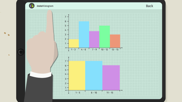
HintsPay attention to the ranges. There are three different types of grouping in ranges.
First look at the lowest and the highest number of pull ups.
It's better to arrange the data in increasing order.
Determine the number of data values in each given range from the histograms.
This number of data values in each range must correspond with the height of the bars.
The total number of people is $6$.
SolutionThe given numbers of pull ups can be ordered:
- $1$
- $4$
- $4$
- $7$
- $9$
- $12$
For a better understanding of given data it's sometimes better to use different ranges.
If we divide the area from $1$ to $12$ in four intervals we get the following
- The number of pull ups from $1$ to $3$ is $1$.
- The number of pull ups from $4$ to $6$ is $2$.
- The number of pull ups from $7$ to $9$ is also $2$.
- The number of pull ups from $10$ to $12$ is $1$ again.
If we divide the area from $1$ to $12$ in three intervals we get the following:
- The number of pull ups from $1$ to $4$ is $3$.
- The number of pull ups from $5$ to $8$ is $1$.
- The number of pull ups from $9$ to $12$ is $2$.
If we divide the area from $1$ to $12$ in two intervals we get the following:
- The number of pull ups from $1$ to $6$ is $3$.
- The number of pull ups from $7$ to $12$ is also $3$.